Exploring the State Papers with Word Embeddings

Last updated on Apr 26, 2021 27 min read

Text and Models

Digital Humanities is often concerned with creating models of text: a general name for a kind of representation of text which makes it in some way easier to interpret. TEI-encoded text is an example of a model: we take the raw material of a text document and add elements to it to make it easier to work with and analyse.

Models are often further abstracted from the original text. One way we can represent text in a way that a machine can interpret is with a word vector. A word vector is simply a numerical representation of a word within a corpus (a body of text, often a series of documents), usually consisting of a series of numbers in a specified sequence. This type of representation is used for a variety of Natural Language Processing tasks - for instance measuring the similarity between two documents.

This post uses a couple of R packages and a method for creating word vectors with a neural net, called GloVe, to produce a series of vectors which give useful clues as to the semantic links between words in a corpus. The method is then used to analyse the printed summaries of the English State Papers, from State Papers Online, and show how they can be used to understand how the association between words and concepts changed over the course of the seventeenth century.

What is a Word Vector, Then?

Imagine you have two documents in a corpus. One of them is an article about pets, and the other is a piece of fiction about a team of crime fighting animal superheroes. We’ll call them document A and document B. One way to represent the words within these documents as a vector would be to use the counts of each word per document.

To do this, you could give each word a set of coordinates, \(x\) and \(y\), where \(x\) is a count of how many times the word appears in document A and \(y\) the number of times it appears in document B.

The first step is to make a dataframe with the relevant counts:

library(ggrepel)
library(tidyverse)
word_vectors = tibble(word = c('crufts', 'feed', 'cat', 'dog', 'mouse', 'rabbit', 'cape', 'hero' ),
      x = c(10, 8, 6, 5, 6, 5, 2, 1),
      y = c(0, 1, 3, 5, 8, 8, 10, 9))

word_vectors

## # A tibble: 8 x 3
##   word       x     y
##   <chr>  <dbl> <dbl>
## 1 crufts    10     0
## 2 feed       8     1
## 3 cat        6     3
## 4 dog        5     5
## 5 mouse      6     8
## 6 rabbit     5     8
## 7 cape       2    10
## 8 hero       1     9

This data can be represented as a two-dimensional plot where each word is placed on the x and y axes based on their x and y values, like this:

ggplot() + 
  geom_point(data = word_vectors, aes(x, y), size =4, alpha = .7) + 
  geom_text_repel(data = word_vectors, aes(x, y, label = word)) + 
  theme_bw() + 
  labs(title = "Words Represented in Two-dimension Space") + 
  theme(title = element_text(face = 'bold')) + 
  scale_x_continuous(breaks = 1:10) + 
  scale_y_continuous(breaks = 1:10)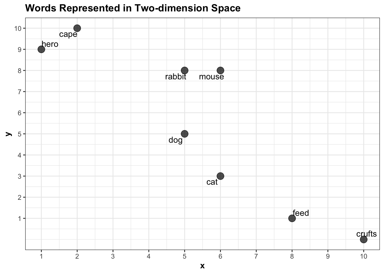

Each word is represented as a vector of length 2: ‘rabbit’ is a vector containing two numbers: {5,8}, for example. Using very basic maths we can calculate the euclidean distance between any pair of words. More or less the only thing I can remember from secondary school math is how to calculate the distance between two points on a graph, using the following formula:

\[ \sqrt {\left( {x_1 - x_2 } \right)^2 + \left( {y_1 - y_2 } \right)^2 } \]

Where \(x\) is the first point and \(y\) the second. This can easily be turned into a function in R, which takes a set of coordinates (the arguments x1 and x2) and returns the euclidean distance:

euc.dist <- function(x1, x2) sqrt(sum((pointA - pointB) ^ 2))

To get the distance between crufts and mouse, set pointA as the \(x\) and \(y\) ccoordinates for the first entry in the dataframe of coordinates we created above, and pointB the coordinates for the fifth entry:

pointA = c(word_vectors$x[1], word_vectors$y[1])
pointB = c(word_vectors$x[5], word_vectors$y[5])

euc.dist(pointA, pointB)

## [1] 8.944272

Representing a pair of words as vectors and measuring the distance between them is commonly used to suggest a semantic link between the two. For instance, the distance between hero and cape in this corpus is small, because they have similar properties: they both occur mostly in the document about superheroes and rarely in the document about pets.

pointA = c(word_vectors$x[word_vectors$word == 'hero'], word_vectors$y[word_vectors$word == 'hero'])

pointB = c(word_vectors$x[word_vectors$word == 'cape'], word_vectors$y[word_vectors$word == 'cape'])

euc.dist(pointA, pointB)

## [1] 1.414214

This suggests that the model has ‘learned’ that in this corpus, hero and cape are semantically more closely linked than other pairs in the dataset. The difference between cape and feed, on the other hand, is large, because one appears often in the superheroes article and rarely in the other, and vice versa.

pointA = c(word_vectors$x[word_vectors$word == 'cape'], word_vectors$y[word_vectors$word == 'cape'])

pointB = c(word_vectors$x[word_vectors$word == 'feed'], word_vectors$y[word_vectors$word == 'feed'])

euc.dist(pointA, pointB)

## [1] 10.81665

Multi-Dimensional Vectors

These vectors, each consisting of two numbers, can be thought of as two-dimensional vectors: a type which can be represented on a 2D scatterplot as \(x\) and \(y\). It’s very easy to add a third dimension, \(z\):

word_vectors_3d = tibble(word = c('crufts', 'feed', 'cat', 'dog', 'mouse', 'rabbit', 'cape', 'hero' ),
      x = c(10, 8, 6, 5, 6, 5, 2, 1),
      y = c(0, 1, 3, 5, 8, 8, 10, 9),
      z = c(1,3,5,2,7,8,4,3))

Just like the plot above, we can plot the words, this time in in three dimensions, using Plotly:

library(plotly)

plot_ly(data = word_vectors_3d, x =  ~x, y = ~y,z =  ~z, text = ~word) %>% add_markers()

You can start to understand how the words now cluster together in the 3D plot: rabbit and mouse are clustered together, but now in the third dimension they are further away from dog. We can use the same formula as above to calculate these distances, just by adding the z coordinates to the pointA and pointB vectors:

pointA = c(word_vectors_3d$x[word_vectors_3d$word == 'dog'], word_vectors_3d$y[word_vectors_3d$word == 'dog'], word_vectors_3d$z[word_vectors_3d$word == 'dog'])
pointB = c(word_vectors_3d$x[word_vectors_3d$word == 'mouse'], word_vectors_3d$y[word_vectors_3d$word == 'mouse'], word_vectors_3d$z[word_vectors_3d$word == 'mouse'])

euc.dist(pointA, pointB)

## [1] 5.91608

The nice thing about the method is that while my brain starts to hurt when I think about more than three dimensions, the maths behind it doesn’t care: you can just keep plugging in longer and longer vectors and it’ll continue to calculate the distances as long as they are the same length. This means you can use this same formula not just when you have x and y coordinates, but also z, a, b, c, d, and so on for as long as you like. This is often called ‘representing words in multi-dimensional euclidean space’, or something similar. Which means that if you represent all the words in a corpus as a long vector (series of coordinates), you can quickly measure the distance between any two.

In a large corpus with a properly-constructed vector representation, the semantic relationships between the words start to make a lot of sense. What’s more, because of vector math, you can add, subtract, divide and multiply the words together to get new vectors, and then find the closest to that. Here, we create a new vector, which is pointA - pointB (dog - mouse). Then loop through each vector and calculate the distance, and display in a new dataframe:

pointC = pointA - pointB

df_for_results = tibble()
for(i in 1:8){
  
  pointA = c(word_vectors_3d$x[i], word_vectors_3d$y[i], word_vectors_3d$z[i])
  u = tibble(dist = euc.dist(pointC, pointA), word = word_vectors_3d$word[i])
  df_for_results = rbind(df_for_results, u)
}

df_for_results %>% arrange(dist)

## # A tibble: 8 x 2
##    dist word  
##   <dbl> <chr> 
## 1  0    mouse 
## 2  1.41 rabbit
## 3  5.39 cat   
## 4  5.39 cape  
## 5  5.92 dog   
## 6  6.48 hero  
## 7  8.31 feed  
## 8 10.8  crufts

We see that the closest to dog minus mouse is hero using this vector representation.

From Vectors to Word Embeddings

These vectors are also known as word embeddings. Real algorithms base the vectors on more sophisticated metrics than that I used above. Some, such as Word2Vec or GloVe, record co-occurrence probabilities (the likelihood of every pair of words in a corpus to co-occur within a set ‘window’ of words either side), using a neural network, and pre-trained over enormous corpora of text. The resulting vectors are often used to represent the relationships between modern meanings of words, to track semantic changes over time, or to understand the history of concepts, though it’s worth pointing out they’re only as representative as the corpus used (many use sources such as Wikipedia, or Reddit, which tend to be produced by privileged and so there’s a danger of biases towards those groups).

Word embeddings are often critiqued as reflecting or propogating bias (I highly recommend Kaspar Beelen’s post and tools to understand more about this) of their source texts. The source used here is a corpus consisting of the printed summaries of the Calendars of State Papers, which I’ve described in detail here. As such it is likely highly biased, but if the purpose of an analysis is historical, for example to understand how a concept was represented at a given time, by a specific group, in a particular body of text, I argue that the biases captured by word embeddings can be seen as a research strength rather than a weakness.

The data is in no way representative of early modern text more generally, and, what’s more, the summaries were written in the 19th century and so will reflect what editors at the time thought was important. In these two ways, the corpus will reproduce a very particular wordview of a very specific group, at a very specific time. Because of this, can use the embeddings to get an idea of how certain words or ideas were semantically linked, specifically in the corpus of calendar abstracts. The data will not show us how early modern concepts were related, but it might help to highlight conceptual changes in words within the information apparatus of the state.

The following instructions are adapted from the text2vec package vignette and this tutorial. First, tokenise all the abstract text and remove very common words called stop words:

library(text2vec)
library(tidytext)
library(textstem)
data("stop_words")
set.seed(1234)

Next, load and pre-process the abstract text:

spo_raw = read_delim('/Users/yannryanpersonal/Documents/blog_posts/MOST RECENT DATA/fromto_all_place_mapped_stuart_sorted', delim = '\t', col_names = F )
spo_mapped_people = read_delim('/Users/yannryanpersonal/Documents/blog_posts/MOST RECENT DATA/people_docs_stuart_200421', delim = '\t', col_names = F)

load('/Users/yannryanpersonal/Documents/blog_posts/g')
g = g %>% group_by(path) %>% summarise(value = paste0(value, collapse = "<br>"))

spo_raw = spo_raw %>%
mutate(X7 = str_replace(X7, "spo", "SPO")) %>%
separate(X7, into = c('Y1', 'Y2', 'Y3'), sep = '/') %>%
mutate(fullpath = paste0("/Users/Yann/Documents/non-Github/spo_xml/", Y1, '/XML/', Y2,"/", Y3)) %>% mutate(uniquecode = paste0("Z", 1:nrow(spo_raw), "Z"))

withtext = left_join(spo_raw, g, by = c('fullpath' = 'path')) %>%
left_join(spo_mapped_people %>% dplyr::select(X1, from_name = X2), by = c('X1' = 'X1'))%>%
left_join(spo_mapped_people %>% dplyr::select(X1, to_name = X2), by = c('X2' = 'X1'))

Tokenize the text using the Tidytext function unnest_tokens(), remove stop words, lemmatize the text (reduce the words to their stem) using textstem, and do a couple of other bits to tidy up. This creates a new dataset, with one row per word - the basis for the algorithm input.

words = withtext %>% 
  ungroup()  %>% 
  select(document = X5, value, date = X3) %>%
  unnest_tokens(word, value) %>% anti_join(stop_words)%>% 
  mutate(word = lemmatize_words(word)) %>% 
  filter(!str_detect(word, "[0-9]{1,}")) %>% mutate(word = str_remove(word, "\\'s"))

Create a ‘vocabulary’, which is just a list of each word found in the dataset and the times they occur, and ‘prune’ it to only include words which occur at least five times.

words_ls = list(words$word)

it = itoken(words_ls, progressbar = FALSE)

vocab = create_vocabulary(it)

vocab = prune_vocabulary(vocab, term_count_min = 5)

With the vocabulary, construct a ‘term co-occurence matrix’: this is a matrix of rows and columns, counting all the times each word co-occurs with every other word, within a window which can be set with the argument skip_grams_window =. 5 seems to give me good results - I think because many of the documents are so short.

vectorizer = vocab_vectorizer(vocab)

# use window of 10 for context words
tcm = create_tcm(it, vectorizer, skip_grams_window = 5)

Now use the GloVe algorithm to train the model and produce the vectors, with a set number of iterations: here we’ve used 20, which seems to give good results. rank here is the number of dimensions we want. x_max is the maximum number of co-occurrences the model will consider in total - giving it a relatively low maximum means that the whole thing won’t be skewed towards a small number of words that occur together hundreds of times. rank sets the number of dimensions in the result. The algorithm can be quite slow, but as it’s a relatively small dataset (in comparison to something like the entire English wikipedia), it shouldn’t take too long to run - a couple of minutes for 20 iterations.

glove = GlobalVectors$new(rank = 100, x_max = 100)

wv_main = glove$fit_transform(tcm, n_iter = 20, convergence_tol = 0.00001)

## INFO  [13:10:58.951] epoch 1, loss 0.0539 
## INFO  [13:11:12.651] epoch 2, loss 0.0318 
## INFO  [13:11:26.593] epoch 3, loss 0.0261 
## INFO  [13:11:40.493] epoch 4, loss 0.0234 
## INFO  [13:11:54.449] epoch 5, loss 0.0217 
## INFO  [13:12:08.337] epoch 6, loss 0.0204 
## INFO  [13:12:22.475] epoch 7, loss 0.0195 
## INFO  [13:12:36.630] epoch 8, loss 0.0187 
## INFO  [13:12:50.738] epoch 9, loss 0.0181 
## INFO  [13:13:04.883] epoch 10, loss 0.0176 
## INFO  [13:13:18.997] epoch 11, loss 0.0172 
## INFO  [13:13:32.954] epoch 12, loss 0.0168 
## INFO  [13:13:46.961] epoch 13, loss 0.0165 
## INFO  [13:14:00.915] epoch 14, loss 0.0162 
## INFO  [13:14:14.873] epoch 15, loss 0.0159 
## INFO  [13:14:28.856] epoch 16, loss 0.0157 
## INFO  [13:14:42.807] epoch 17, loss 0.0155 
## INFO  [13:14:56.780] epoch 18, loss 0.0153 
## INFO  [13:15:10.708] epoch 19, loss 0.0151 
## INFO  [13:15:24.759] epoch 20, loss 0.0149

GloVe results in two sets of word vectors, the main and the context. The authors of the GloVe package suggest that combining both results in higher-quality embeddings:

wv_context = glove$components



# Either word-vectors matrices could work, but the developers of the technique
# suggest the sum/mean may work better
word_vectors = wv_main + t(wv_context)

Reducing Dimensionality for Visualisation

Now that’s done, it’d be nice to visualise the results as a whole. This isn’t actually necessary: as I mentioned earlier, the computer doesn’t care how many dimensions you give it to work out the distances between words. However, in order to visualise the results, we can reduce the 100 dimensions to two or three and plot the results. We can do this with an algorithm called UMAP

There are a number of parameters which can be set - most important is n_components, the number of dimensions, which should be set to two or three so that the results can be plotted.

library(umap)
glove_umap <- umap(word_vectors, n_components = 3, metric = "cosine", n_neighbors = 25, min_dist = 0.01, spread=2)

df_glove_umap <- as.data.frame(glove_umap$layout, stringsAsFactors = FALSE)

# Add the labels of the words to the dataframe
df_glove_umap$word <- rownames(df_glove_umap)
colnames(df_glove_umap) <- c("UMAP1", "UMAP2", "UMAP3", "word")

Next, use Plotly as above to visualise the resulting three dimensions:

plot_ly(data = df_glove_umap, x =  ~UMAP1, y = ~UMAP2, z =  ~UMAP3, text = ~word, alpha = .2, size = .1) %>% add_markers(mode = 'text')

The resulting 3D scatterplot (very happy I actually managed to use one appropriately) can be used to explore how words are related in the State Papers corpus. You can pan and zoom through the plot using the mouse, which will show clusters of (sometimes) logically related words. My favourite so far is a large, outlying cluster of ‘weather’ words like gale, snow, storm, etc: many of the correspondents writing to the Secretary of State Joseph Williamson would send regular weather reports alongside local and international news.

Results

In order to more easily explore the results, write a small function which calculates and displays the closest words in distance to a given word. Instead of using the euclidean distance formula above, we calculate the cosine similarity, which measures the angular distance between the words (this is better because it corrects for one word appearing many times and another appearing very infrequently).

closest_words = function(word){

word_result = word_vectors[word, , drop = FALSE] 

cos_sim = sim2(x = word_vectors, y = word_result, method = "cosine", norm = "l2")


head(sort(cos_sim[,1], decreasing = TRUE), 30)

}

The function takes a single word as an argument and returns the twenty closest word vectors, by cosine distance. What are the closest in useage to ‘king’?

closest_words('king')

##       king    majesty      queen    england     desire       lord       late 
##  1.0000000  0.8608965  0.7623216  0.7574458  0.7320683  0.7291221  0.7275582 
## understand     please    command      leave       time       hope     prince 
##  0.7249386  0.7174364  0.7167840  0.7142780  0.7133477  0.7132760  0.7131191 
##    receive     letter     intend      grant     inform       hear    promise 
##  0.7116103  0.7090872  0.7085671  0.7085476  0.7073241  0.7037661  0.7036833 
##       duke    service     favour       pray       tell      offer     return 
##  0.7008882  0.6992494  0.6990657  0.6973842  0.6900713  0.6886157  0.6883724 
##      bring       earl 
##  0.6870097  0.6800224

Unsurprisingly, a word that is often interchangeable with King, Majesty, is the closest, followed by ‘Queen’ - also obviously interchangeable with King, depending on the circumstances.

Word embeddings are often used to understand different and changing gender representations. How are gendered words represented in the State Papers abstracts? First of all, wife:

closest_words('wife')

##      wife     child   husband    sister  daughter     marry    mother      lady 
## 1.0000000 0.8345385 0.7816025 0.7800919 0.7351106 0.7270973 0.7254064 0.7216592 
##    father   brother       son    family     widow     woman   servant    friend 
## 0.7167650 0.7164700 0.7028317 0.6767484 0.6641016 0.6515075 0.6351253 0.6336372 
##     leave      poor      live      life     uncle    writer     niece       die 
## 0.5945169 0.5883705 0.5779839 0.5771607 0.5750166 0.5746008 0.5687118 0.5631986 
##      pray      dead       beg  remember    estate    health 
## 0.5630201 0.5579240 0.5478639 0.5447117 0.5373690 0.5323630

Unsurprisingly wife is most similar to other words relating to family. What about husband?

closest_words('husband')

##      husband         wife        child        widow      servant   petitioner 
##    1.0000000    0.7816025    0.7380409    0.6775940    0.6474966    0.6281474 
##        woman       father         debt         lady       sister       mother 
##    0.6278084    0.6221267    0.6163868    0.6031975    0.5861202    0.5812222 
##         late     daughter       family     prisoner      brother        marry 
##    0.5756477    0.5746393    0.5743044    0.5726222    0.5702953    0.5699526 
##          son       access          die      release     petition      decease 
##    0.5676153    0.5647356    0.5598512    0.5578828    0.5573955    0.5570279 
## imprisonment          beg         pray        death       suffer         poor 
##    0.5484621    0.5270811    0.5261175    0.5218034    0.5159048    0.5084243

Husband is mostly similar but with some interesting different associations: ‘widow’, ‘die’, ‘petition’, ‘debt’, and ‘prisoner’, reflecting the fact that there is a large group of petitions in the State Papers written by women looking for pardons or clemency for their husbands, particularly following the Monmouth Rebellion in 1683.

Looking at the closest words to place names gives some interesting associations. Amsterdam is associated with terms related to shipping and trade:

closest_words('amsterdam')

##   amsterdam   rotterdam        lade    merchant        bind     hamburg 
##   1.0000000   0.7666191   0.6215717   0.5732498   0.5710452   0.5608900 
##    bordeaux       prize     holland      vessel    dutchman      richly 
##   0.5516391   0.5485984   0.5433259   0.5414728   0.5320493   0.5112544 
##       dutch      french        salt     zealand      london         hoy 
##   0.5039151   0.5032062   0.5014527   0.4992265   0.4969952   0.4915483 
##       flush        port      france   privateer   frenchman      arrive 
##   0.4843777   0.4781653   0.4774213   0.4768828   0.4729506   0.4725824 
##      ostend    hamburgh      lisbon        ship      nantes merchantmen 
##   0.4711110   0.4703833   0.4696365   0.4673227   0.4649912   0.4631832

Whereas Rome is very much associated with religion and ecclesiastical politics:

closest_words('rome')

##        rome        pope      jesuit       spain    cardinal       paris 
##   1.0000000   0.6403637   0.5744878   0.5533940   0.5512975   0.5275787 
##      priest      venice       italy      naples     courier       friar 
##   0.5113264   0.5025585   0.4814730   0.4771853   0.4727892   0.4722075 
##     germany      nuncio     england      tyrone        doge        mass 
##   0.4688932   0.4544449   0.4523312   0.4513841   0.4482686   0.4482273 
##  ambassador     primate      france    catholic inquisition    archduke 
##   0.4478178   0.4442790   0.4376338   0.4324462   0.4208505   0.4182811 
##   archdukes    dominion      church      banish      vienna    brussels 
##   0.4116746   0.4069731   0.4064238   0.4040390   0.4025671   0.3952721

More Complex Vector Tasks

As well as finding the most similar words, we can also perform arithmetic on the vectors. What is the closest word to book plus news?

sum = word_vectors["book", , drop = F] +
 word_vectors["news", , drop = F]

cos_sim_test = sim2(x = word_vectors, y = sum, method = "cosine", norm = "l2")

head(sort(cos_sim_test[,1], decreasing = T), 20)

##       news       book       send    account     letter      write       hear 
##  0.8135916  0.7994320  0.6786464  0.6769291  0.6712663  0.6566995  0.6561809 
##      bring       post williamson        day    enclose    receive      print 
##  0.6465319  0.6449987  0.6418133  0.6390539  0.6337941  0.6308958  0.6240721 
##       hope     return       note     expect       hand       time 
##  0.6191154  0.6180249  0.6180092  0.6080522  0.6072797  0.6059994

It is also a way of finding analogies: so, for example, Paris - France + Germany should equal to ‘Berlin’, because Berlin is like the Paris of France. Is that what we get?

test = word_vectors["paris", , drop = F] -
  word_vectors["france", , drop = F] +
  word_vectors["germany", , drop = F]
  
#+
 # shakes_word_vectors["letter", , drop = F]

cos_sim_test = sim2(x = word_vectors, y = test, method = "cosine", norm = "l2")

head(sort(cos_sim_test[,1], decreasing = T), 20)

##         paris       germany            ps      brussels           n.s 
##     0.6591308     0.6105675     0.4884733     0.4704956     0.4691332 
##         style         hague         early advertisement       edmonds 
##     0.4682669     0.4679999     0.4216780     0.4014141     0.3936226 
##         cover           thy complimentary        madrid    occurrence 
##     0.3893444     0.3892593     0.3874887     0.3826021     0.3810840 
##        digest        eugene       majeste     frankfort         often 
##     0.3800077     0.3743125     0.3729503     0.3716548     0.3691617

Not quite. After Germany and Paris and some auxiliary words (N.S. and style are related to different calendar systems and they frequently occur with locations because writers often stated which they were using to avoid confusion) the most similar to Paris - France + Germany is Brussels: not the correct answer, but a close enough guess! There are also many other capital cities in the top twenty.

We can try other analogies: pen - letter + book should in theory give some word related to printing and book production such as print, or press, or maybe type (Think pen is to letter as X is to book).

test = word_vectors["pen", , drop = F] -
  word_vectors["letter", , drop = F] +
    word_vectors["book", , drop = F]
  
cos_sim_test = sim2(x = word_vectors, y = test, method = "cosine", norm = "l2")

head(sort(cos_sim_test[,1], decreasing = T), 20)

##        pen   pamphlet       book        ink manuscript unlicensed     physic 
##  0.5311813  0.5102215  0.4989869  0.4929565  0.4681780  0.4610147  0.4377186 
##     closet bookseller      bible     quires    printer        dig traitorous 
##  0.4324101  0.4201757  0.4192146  0.4137985  0.4090402  0.4054834  0.3983979 
##   dedicate    avebury      study      super     author       sowe 
##  0.3883951  0.3828235  0.3801104  0.3798285  0.3796215  0.3792047

Not bad - printer is in the top 20! The closest is ink, plus some other book-production-related words like pamphlet. Though some of these words can also be associated with manuscript production, we could be generous and say that they are sort of to a book as a pen is to a letter!

Change in Semantic Relations Over Time

We can also look for change in semantic meaning over time. First, divide the text into four separate sections, one for each reign:

library(lubridate)
james_i = withtext %>% 
  mutate(year = year(ymd(X4))) %>% 
  filter(year %in% 1603:1624) %>% 
  ungroup()  %>% 
  select(document = X5, value, date = X3) %>%
  unnest_tokens(word, value) %>% 
  anti_join(stop_words) %>% 
  mutate(word = lemmatize_words(word)) %>% filter(!str_detect(word, "[0-9]{1,}"))

charles_i = withtext %>% 
  mutate(year = year(ymd(X4))) %>% 
  filter(year %in% 1625:1648) %>% 
  ungroup()  %>% 
  select(document = X5, value, date = X3) %>%
  unnest_tokens(word, value) %>% anti_join(stop_words)%>% 
  mutate(word = lemmatize_words(word)) %>% filter(!str_detect(word, "[0-9]{1,}"))

commonwealth = withtext %>% 
  mutate(year = year(ymd(X4))) %>% 
  filter(year %in% 1649:1659) %>% 
  ungroup()  %>% 
  select(document = X5, value, date = X3) %>%
  unnest_tokens(word, value) %>% anti_join(stop_words)%>% 
  mutate(word = lemmatize_words(word)) %>% filter(!str_detect(word, "[0-9]{1,}"))

charles_ii = withtext %>% 
  mutate(year = year(ymd(X4))) %>% 
  filter(year %in% 1660:1684) %>% 
  ungroup()  %>% 
  select(document = X5, value, date = X3) %>%
  unnest_tokens(word, value) %>% anti_join(stop_words)%>% 
  mutate(word = lemmatize_words(word)) %>% filter(!str_detect(word, "[0-9]{1,}"))

james_ii_w_m_ann = withtext %>% 
  mutate(year = year(ymd(X4))) %>% 
  filter(year %in% 1685:1714) %>% 
  ungroup()  %>% 
  select(document = X5, value, date = X3) %>%
  unnest_tokens(word, value) %>% anti_join(stop_words) %>% 
  mutate(word = lemmatize_words(word)) %>% filter(!str_detect(word, "[0-9]{1,}"))

Now run the same scripts as above, on each of these sections:

james_i_words_ls = list(james_i$word)
it = itoken(james_i_words_ls, progressbar = FALSE)
james_i_vocab = create_vocabulary(it)
james_i_vocab = prune_vocabulary(james_i_vocab, term_count_min = 5)

vectorizer = vocab_vectorizer(james_i_vocab)

# use window of 10 for context words
james_i_tcm = create_tcm(it, vectorizer, skip_grams_window = 5)

james_i_glove = GlobalVectors$new(rank = 100, x_max = 100)

james_i_wv_main = james_i_glove$fit_transform(james_i_tcm, n_iter = 20, convergence_tol = 0.00001)

## INFO  [13:20:40.350] epoch 1, loss 0.0496 
## INFO  [13:20:43.722] epoch 2, loss 0.0291 
## INFO  [13:20:47.094] epoch 3, loss 0.0231 
## INFO  [13:20:50.476] epoch 4, loss 0.0203 
## INFO  [13:20:53.852] epoch 5, loss 0.0185 
## INFO  [13:20:57.211] epoch 6, loss 0.0172 
## INFO  [13:21:00.588] epoch 7, loss 0.0162 
## INFO  [13:21:03.919] epoch 8, loss 0.0154 
## INFO  [13:21:07.317] epoch 9, loss 0.0147 
## INFO  [13:21:10.663] epoch 10, loss 0.0142 
## INFO  [13:21:14.032] epoch 11, loss 0.0137 
## INFO  [13:21:17.384] epoch 12, loss 0.0132 
## INFO  [13:21:20.743] epoch 13, loss 0.0129 
## INFO  [13:21:24.100] epoch 14, loss 0.0125 
## INFO  [13:21:27.453] epoch 15, loss 0.0122 
## INFO  [13:21:30.839] epoch 16, loss 0.0120 
## INFO  [13:21:34.283] epoch 17, loss 0.0117 
## INFO  [13:21:37.665] epoch 18, loss 0.0115 
## INFO  [13:21:41.097] epoch 19, loss 0.0113 
## INFO  [13:21:44.465] epoch 20, loss 0.0111

james_i_wv_context = james_i_glove$components

james_i_word_vectors = james_i_wv_main + t(james_i_wv_context)

charles_i_words_ls = list(charles_i$word)
it = itoken(charles_i_words_ls, progressbar = FALSE)
charles_i_vocab = create_vocabulary(it)
charles_i_vocab = prune_vocabulary(charles_i_vocab, term_count_min = 5)

vectorizer = vocab_vectorizer(charles_i_vocab)

# use window of 10 for context words
charles_i_tcm = create_tcm(it, vectorizer, skip_grams_window = 5)

charles_i_glove = GlobalVectors$new(rank = 100, x_max = 100)

charles_i_wv_main = charles_i_glove$fit_transform(charles_i_tcm, n_iter = 20, convergence_tol = 0.00001)

## INFO  [13:21:54.036] epoch 1, loss 0.0533 
## INFO  [13:21:58.232] epoch 2, loss 0.0298 
## INFO  [13:22:02.444] epoch 3, loss 0.0234 
## INFO  [13:22:06.649] epoch 4, loss 0.0207 
## INFO  [13:22:10.890] epoch 5, loss 0.0189 
## INFO  [13:22:15.137] epoch 6, loss 0.0176 
## INFO  [13:22:19.423] epoch 7, loss 0.0166 
## INFO  [13:22:23.683] epoch 8, loss 0.0158 
## INFO  [13:22:27.949] epoch 9, loss 0.0152 
## INFO  [13:22:32.178] epoch 10, loss 0.0146 
## INFO  [13:22:36.395] epoch 11, loss 0.0141 
## INFO  [13:22:40.576] epoch 12, loss 0.0137 
## INFO  [13:22:44.766] epoch 13, loss 0.0134 
## INFO  [13:22:48.984] epoch 14, loss 0.0130 
## INFO  [13:22:53.287] epoch 15, loss 0.0127 
## INFO  [13:22:57.572] epoch 16, loss 0.0125 
## INFO  [13:23:01.768] epoch 17, loss 0.0122 
## INFO  [13:23:05.947] epoch 18, loss 0.0120 
## INFO  [13:23:10.131] epoch 19, loss 0.0118 
## INFO  [13:23:14.333] epoch 20, loss 0.0116

charles_i_wv_context = charles_i_glove$components

charles_i_word_vectors = charles_i_wv_main + t(charles_i_wv_context)

commonwealth_words_ls = list(commonwealth$word)
it = itoken(commonwealth_words_ls, progressbar = FALSE)
commonwealth_vocab = create_vocabulary(it)
commonwealth_vocab = prune_vocabulary(commonwealth_vocab, term_count_min = 5)

vectorizer = vocab_vectorizer(commonwealth_vocab)

# use window of 10 for context words
commonwealth_tcm = create_tcm(it, vectorizer, skip_grams_window = 5)

commonwealth_glove = GlobalVectors$new(rank = 100, x_max = 100)

commonwealth_wv_main = commonwealth_glove$fit_transform(commonwealth_tcm, n_iter = 20, convergence_tol = 0.00001)

## INFO  [13:23:18.408] epoch 1, loss 0.0555 
## INFO  [13:23:20.221] epoch 2, loss 0.0319 
## INFO  [13:23:21.989] epoch 3, loss 0.0248 
## INFO  [13:23:23.735] epoch 4, loss 0.0215 
## INFO  [13:23:25.478] epoch 5, loss 0.0194 
## INFO  [13:23:27.226] epoch 6, loss 0.0178 
## INFO  [13:23:28.970] epoch 7, loss 0.0167 
## INFO  [13:23:30.717] epoch 8, loss 0.0157 
## INFO  [13:23:32.466] epoch 9, loss 0.0150 
## INFO  [13:23:34.229] epoch 10, loss 0.0143 
## INFO  [13:23:35.990] epoch 11, loss 0.0138 
## INFO  [13:23:37.742] epoch 12, loss 0.0133 
## INFO  [13:23:39.486] epoch 13, loss 0.0128 
## INFO  [13:23:41.234] epoch 14, loss 0.0125 
## INFO  [13:23:42.982] epoch 15, loss 0.0121 
## INFO  [13:23:44.730] epoch 16, loss 0.0118 
## INFO  [13:23:46.481] epoch 17, loss 0.0115 
## INFO  [13:23:48.228] epoch 18, loss 0.0113 
## INFO  [13:23:49.977] epoch 19, loss 0.0110 
## INFO  [13:23:51.744] epoch 20, loss 0.0108

commonwealth_wv_context = commonwealth_glove$components

# dim(shakes_wv_context)

# Either word-vectors matrices could work, but the developers of the technique
# suggest the sum/mean may work better
commonwealth_word_vectors = commonwealth_wv_main + t(commonwealth_wv_context)

charles_ii_words_ls = list(charles_ii$word)
it = itoken(charles_ii_words_ls, progressbar = FALSE)
charles_ii_vocab = create_vocabulary(it)
charles_ii_vocab = prune_vocabulary(charles_ii_vocab, term_count_min = 5)

vectorizer = vocab_vectorizer(charles_ii_vocab)

# use window of 10 for context words
charles_ii_tcm = create_tcm(it, vectorizer, skip_grams_window = 5)

charles_ii_glove = GlobalVectors$new(rank = 100, x_max = 100)

charles_ii_wv_main = charles_ii_glove$fit_transform(charles_ii_tcm, n_iter = 20, convergence_tol = 0.00001)

## INFO  [13:24:05.888] epoch 1, loss 0.0506 
## INFO  [13:24:12.307] epoch 2, loss 0.0288 
## INFO  [13:24:18.627] epoch 3, loss 0.0232 
## INFO  [13:24:25.022] epoch 4, loss 0.0205 
## INFO  [13:24:31.320] epoch 5, loss 0.0189 
## INFO  [13:24:37.617] epoch 6, loss 0.0176 
## INFO  [13:24:44.006] epoch 7, loss 0.0167 
## INFO  [13:24:50.331] epoch 8, loss 0.0160 
## INFO  [13:24:56.655] epoch 9, loss 0.0154 
## INFO  [13:25:02.993] epoch 10, loss 0.0149 
## INFO  [13:25:09.405] epoch 11, loss 0.0144 
## INFO  [13:25:15.778] epoch 12, loss 0.0140 
## INFO  [13:25:22.122] epoch 13, loss 0.0137 
## INFO  [13:25:28.438] epoch 14, loss 0.0134 
## INFO  [13:25:34.735] epoch 15, loss 0.0131 
## INFO  [13:25:41.037] epoch 16, loss 0.0129 
## INFO  [13:25:47.361] epoch 17, loss 0.0127 
## INFO  [13:25:53.700] epoch 18, loss 0.0125 
## INFO  [13:26:00.002] epoch 19, loss 0.0123 
## INFO  [13:26:06.318] epoch 20, loss 0.0121

charles_ii_wv_context = charles_ii_glove$components

# dim(shakes_wv_context)

# Either word-vectors matrices could work, but the developers of the technique
# suggest the sum/mean may work better
charles_ii_word_vectors = charles_ii_wv_main + t(charles_ii_wv_context)

james_ii_w_m_ann_words_ls = list(james_ii_w_m_ann$word)
it = itoken(james_ii_w_m_ann_words_ls, progressbar = FALSE)
james_ii_w_m_ann_vocab = create_vocabulary(it)
james_ii_w_m_ann_vocab = prune_vocabulary(james_ii_w_m_ann_vocab, term_count_min = 5)

vectorizer = vocab_vectorizer(james_ii_w_m_ann_vocab)

# use window of 10 for context words
james_ii_w_m_ann_tcm = create_tcm(it, vectorizer, skip_grams_window = 5)

james_ii_w_m_ann_glove = GlobalVectors$new(rank = 100, x_max = 100)

james_ii_w_m_ann_wv_main = james_ii_w_m_ann_glove$fit_transform(james_ii_w_m_ann_tcm, n_iter = 20, convergence_tol = 0.00001)

## INFO  [13:26:12.288] epoch 1, loss 0.0516 
## INFO  [13:26:15.088] epoch 2, loss 0.0295 
## INFO  [13:26:17.865] epoch 3, loss 0.0235 
## INFO  [13:26:20.639] epoch 4, loss 0.0207 
## INFO  [13:26:23.407] epoch 5, loss 0.0188 
## INFO  [13:26:26.180] epoch 6, loss 0.0174 
## INFO  [13:26:28.951] epoch 7, loss 0.0164 
## INFO  [13:26:31.728] epoch 8, loss 0.0156 
## INFO  [13:26:34.490] epoch 9, loss 0.0149 
## INFO  [13:26:37.261] epoch 10, loss 0.0143 
## INFO  [13:26:40.030] epoch 11, loss 0.0138 
## INFO  [13:26:42.796] epoch 12, loss 0.0133 
## INFO  [13:26:45.568] epoch 13, loss 0.0129 
## INFO  [13:26:48.339] epoch 14, loss 0.0126 
## INFO  [13:26:51.102] epoch 15, loss 0.0123 
## INFO  [13:26:53.869] epoch 16, loss 0.0120 
## INFO  [13:26:56.634] epoch 17, loss 0.0117 
## INFO  [13:26:59.403] epoch 18, loss 0.0115 
## INFO  [13:27:02.176] epoch 19, loss 0.0113 
## INFO  [13:27:04.942] epoch 20, loss 0.0111

james_ii_w_m_ann_wv_context = james_ii_w_m_ann_glove$components

# dim(shakes_wv_context)

# Either word-vectors matrices could work, but the developers of the technique
# suggest the sum/mean may work better
james_ii_w_m_ann_word_vectors = james_ii_w_m_ann_wv_main + t(james_ii_w_m_ann_wv_context)

Write a function as above, this time with two arguments, so we can specify both the word and the relevant reign:

top_ten_function = function(word, period){
  
  
  if(period == 'james_i'){
    
  vectors = james_i_word_vectors[word, , drop = FALSE] 
  cos_sim = sim2(x = james_i_word_vectors, y = vectors, method = "cosine", norm = "l2")


}
  else if(period == 'charles_i'){  vectors = charles_i_word_vectors[word, , drop = FALSE] 
  cos_sim = sim2(x = charles_i_word_vectors, y = vectors, method = "cosine", norm = "l2")
  
  } 
  else if(period == 'commonwealth')  { 
    
    vectors = commonwealth_word_vectors[word, , drop = FALSE] 
  cos_sim = sim2(x = commonwealth_word_vectors, y = vectors, method = "cosine", norm = "l2")
  
  }
  
  else if(period == 'charles_ii'){
    
    vectors = charles_ii_word_vectors[word, , drop = FALSE] 
  cos_sim = sim2(x = charles_ii_word_vectors, y = vectors, method = "cosine", norm = "l2")
  
  }
  
  else {
    
  vectors = james_ii_w_m_ann_word_vectors[word, , drop = FALSE] 
  cos_sim = sim2(x = james_ii_w_m_ann_word_vectors, y = vectors, method = "cosine", norm = "l2")
  }
  
head(sort(cos_sim[,1], decreasing = TRUE), 20)


}

Write a second function, which takes a word and returns the ten closest words for each reign:

first_in_each= function(word) {
  
  rbind(top_ten_function(word, 'james_i') %>% tibble::enframe() %>% arrange(desc(value)) %>% slice(2:11) %>% mutate(reign ='james_i' ),
     top_ten_function(word, 'charles_i') %>% tibble::enframe() %>% arrange(desc(value)) %>% slice(2:11) %>% mutate(reign ='charles_i' ),
     top_ten_function(word, 'commonwealth') %>% tibble::enframe() %>% arrange(desc(value)) %>% slice(2:11) %>% mutate(reign ='commonwealth' ),
     top_ten_function(word, 'charles_ii') %>% tibble::enframe() %>% arrange(desc(value)) %>% slice(2:11) %>% mutate(reign ='charles_ii' ),
     top_ten_function(word, 'james_ii_w_m_ann') %>% tibble::enframe() %>% arrange(desc(value)) %>% slice(2:11) %>% mutate(reign ='james_ii_w_m_ann' ))%>% 
  group_by(reign) %>% 
  mutate(rank = rank(value)) %>% 
  ggplot() + 
  geom_text(aes(x = factor(reign, levels = c('james_i', 'charles_i', 'commonwealth', 'charles_ii', 'james_ii', 'james_ii_w_m_ann')), y = rank, label = name, color = name)) + theme_void() +
  theme(legend.position = 'none', 
        axis.text.x = element_text(face = 'bold'), 
        ) 
  
  }

This can show us the changing associations of particular words over time. Take ‘match’:

first_in_each('match')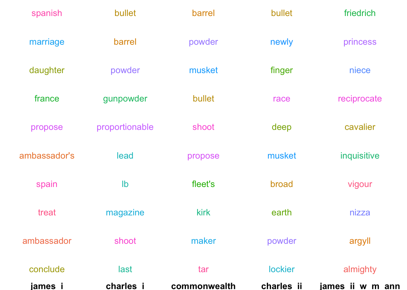

In the reign of James I, ‘match’ is semantically linked to words relating to the Spanish Match: a proposed match between Charles I and the Infanta Maria Anna of Spain. During Charles I’s reign and afterwards, the meaning changes completely - now the closest words are all related to guns and cannons—unsurprising for a period marked by warfare right across Europe. In the final section of the data, the semantic link changes again - though this time it’s not so obvious how the related words are associated.

Conclusions

The primary purpose of this technique in the ‘real world’ isn’t really to understand the semantic relationship between words for its own sake, but rather is most often used as part of an NLP pipeline, where the embeddings are fed through a neural net to make predictions about text.

However, the word embeddings trained on the text of the Calendars is still a useful way to think about how these texts are constructed and the sort of ‘mental map’ they represent. We’ve seen that it often produces expected results (such as King being closest to Majesty), even in complex tasks: with the analogy pen is to letter as X is to book, X is replaced by ink, printer, pamphlet, and some other relevant book-production words. Certain words can be seen to change over time: match is a good example, which is linked to marriage at some times, and weaponry at others, depending on the time period.

Many of these word associations reflect biases in the data, but in certain circumstances this can be a strength rather than a weakness. The danger is not investigating the biases, but rather when we are reductive and try to claim that the word associations seen here are in any way representative of how society at large thought about these concepts more generally. On their own terms, the embeddings can be a powerful historical tool to understand the linked meanings within a discrete set of sources.