Early modern routing with Viabundus and sfnetworks

The last couple of months have been particularly good ones for anyone working with spatial and historical data: An major new ‘online streetmap’ of early modern Northern Europe, Viabundus, was released at the end of April, about a month after the first CRAN release of an R package called sfnetworks. This package and dataset seem made for each other: with some pretty basic code I’ve been able to do some really fun things.
sfnetworks package
The stnetworks package has been in development for some time, but the first I heard of it was in March when they announced the first CRAN release (which means it’s in R’s ‘official’ list of packages that can be installed through the programming language itself). Essentially, two of my favourite packages, sf for spatial analysis and tidygraph for networks, have got together and had a baby: sfnetworks combines both packages, providing a really easy interface for performing spatial network analysis tasks such as calculating shortest paths.
As I wrote in an earlier post, tidygraph allows you to perform network analysis within a tidy data workflow, by linking together a nodes table and an edges table, allows you to switch between the two and easily do typical data analysis tasks such as grouping and filtering, directly to the network itself.
sfnetworks extends this idea by making the nodes and edges tables into simple features spatial objects: the nodes table becomes a table of spatial points, and the edges table one of spatial lines. You can also just supply one or the other and it’ll automatically make the second - so for example if you supply a table of spatial points, it’ll draw implicit edges between them, and, conversely, if you supply a dataset of spatial lines, it’ll give you a table of nodes, consisting of all the start and end points of each of the lines. Simple features objects are particularly easy to work with thanks to the R package sf: the sfnetworks format lets you leverage all the great GIS analysis from sf along with network-specific tasks.
The examples below are all based on the package vignettes and the result of a couple of days playing around. I highly recommend taking a look at these to understand the full data structure - which I have simplified and, I’m sure in parts, misunderstood.
Viabundus
As luck would have it, the data type needed for sfnetworks is pretty similar to the second resource I mentioned, Viabundus. Viabundus is the result of a four-year project by a group of researchers in Universities across Europe, which the creators describe as a ‘online street map of late medieval and early modern northern Europe (1350-1650).’ It’s an atlas of early modern roads, which have been digitised and converted into a nifty online map which allows you to calculate routes across Northern Europe, including travel times, tolls passed, fairs visited, to a pretty mind-boggling level of detail. Basically Google Maps for the seventeenth-century.
Alongside the map, the team have released the dataset as Open Access (CC-BY-SA) data. There’s extensive documentation, but in essence, to reconstruct the basic map and perform spatial analysis with it, the data contains two key tables: one edges table, the roads, and one nodes table, the towns, markets, bridges and other points through which the routes pass. As I said - conveniently this is more or less the data structure required as an input for sfnetworks. The rest of this post is a short demonstration on how the two can be used together.
Create a sfnetworks object from Viabundus data
The data is freely available here, with a CC-BY-SA licence. I recommend having a good read of the documentation to understand all the additional tables, but the ones we’ll use today are the two main ones: the nodes and edges. First, import them into R:
library(tidyverse)
nodes = read_csv('Viabundus-1.0-CSV/Nodes.csv')
edges = read_csv('Viabundus-1.0-CSV/Edges.csv')
Next, you need to convert them into sf objects. The geographic data in the Viabundus edges table is supplied in a format called ‘Well Known Text’ (WKT). The sf package supports this as a data input - just supply the column containing the spatial data as the argument wkt =. In this case, the WKT column in the edges table is also called WKT. Use st_set_crs to set the Coordinate Reference System, which needs to be the same for both tables.
library(sf)
edges_sf = edges %>% st_as_sf(wkt = "WKT")
edges_sf = edges_sf %>% st_set_crs(4326)
The nodes table doesn’t use WKT, but contains a regular latitude and longitude column. Use st_as_sf again, and supply the column names to the coords = argument.
nodes_sf = nodes %>% st_as_sf(coords = c('Longitude', 'Latitude'))
nodes_sf = nodes_sf %>% st_set_crs(4326)
To create the sfnetworks object, you supply data in one of a number of forms. The most complete is to supply a both a table of edges and a table of nodes. The edges table should contain ‘from’ and ‘to’ columns, corresponding to the node IDs in the node table, which will link them together.
As far as I can tell, the Viabundus data doesn’t explicitly connect the nodes and edges data like this. I’ve used a sort of work-around to get around this.
First, use as_sfnetwork to create an sfnetwork from the edges table alone.
library(sfnetworks)
sf_net = as_sfnetwork(edges_sf, directed = F)

sf_net
## # A sfnetwork with 12567 nodes and 14819 edges
## #
## # CRS:  EPSG:4326
## #
## # An undirected multigraph with 10 components with spatially explicit edges
## #
## # Node Data:     12,567 x 1 (active)
## # Geometry type: POINT
## # Dimension:     XY
## # Bounding box:  xmin: 3.224534 ymin: 48.72051 xmax: 37.6206 ymax: 60.71302
##                   WKT
##           <POINT [°]>
## 1 (22.47944 58.24702)
## 2 (22.80928 58.30961)
## 3 (22.86145 58.36151)
## 4 (23.00004 58.40795)
## 5  (23.04775 58.5087)
## 6 (23.03553 58.57549)
## # … with 12,561 more rows
## #
## # Edge Data:     14,819 x 12
## # Geometry type: LINESTRING
## # Dimension:     XY
## # Bounding box:  xmin: 3.222333 ymin: 48.72051 xmax: 37.6206 ymax: 60.71302
##    from    to     ID Section Type  Certainty Zoomlevel From  To    Comment_ID
##   <int> <int>  <dbl> <chr>   <chr>     <dbl>     <dbl> <chr> <chr> <chr>
## 1     1     2 227856 EST     land          2         1 NULL  NULL  NULL
## 2     2     3 227858 EST     land          2         1 NULL  NULL  NULL
## 3     3     4 227860 EST     land          3         1 NULL  NULL  NULL
## # … with 14,816 more rows, and 2 more variables: Length <dbl>, WKT <LINESTRING
## #   [°]>
Looking at the data, you can see it has created a simple nodes table of all the start and end points of the spatial lines in the edges table. We need to know what towns and other points correspond to these nodes.
To do this, I used the sf function st_join. Use the join function ‘nearest feature,’ which will link the sfnetwork nodes table to the closest point in the original Viabundus nodes table. This is the best method I could think of for now, though it’s not perfect—it would be better if there was an explicit link between the nodes and edges table, which I haven’t been able to figure out.
sf_net = sf_net %>%
  st_join(nodes_sf, join = st_nearest_feature)
One of the key things which makes a spatial network object different to a regular network object is that we treat the length of each edge as a weight. This can be done automatically with sfnetworks using edge_length, though the Viabundus edges table has a column with this information already.
sf_net = sf_net %>%
  activate("edges") %>%
  mutate(weight = edge_length())
Network Calculations
This new object can be used to calculate regular network analysis metrics, such as betweenness centrality, using the same set of functions as tidygraph:
library(tidygraph)
library(kableExtra)
betweenness_scores = sf_net %>%
  activate(nodes) %>%
  mutate(betweenness = centrality_betweenness(weights = NULL)) %>%
  as_tibble() %>%
  arrange(desc(betweenness)) %>%
  filter(Is_Town == 'y') %>% head(10)

betweenness_scores %>% st_drop_geometry() %>% select(Name, betweenness) %>% kbl(caption = "Nodes with highest betweenness scores:")
| Name | betweenness |
|---|---|
| Wittenberge | 21883786 |
| Cölln (Berlin) | 21044547 |
| Havelberg | 20997097 |
| Hitzacker | 20414717 |
| Berlin | 19693706 |
| Berlin | 19316790 |
| Bernau bei Berlin | 19291164 |
| Potsdam | 19272557 |
| Bernau bei Berlin | 19257977 |
| Malchow | 19240900 |
Or color all nodes on their betweenness score, and display on a map:
betweenness_sf = sf_net %>%
  activate(nodes) %>%
  mutate(betweenness = centrality_betweenness(weights = NULL)) %>%
  as_tibble()

ggplot() + geom_sf(data = betweenness_sf, aes(color = betweenness), alpha =  .8) + scale_color_viridis_c() +theme_void() + labs(title  = "Viabundus Network, Betweenness Centrality Scores", caption = 'Made with data from Viabundus.eu') + theme(title = element_text(size = 14, face = 'bold'))
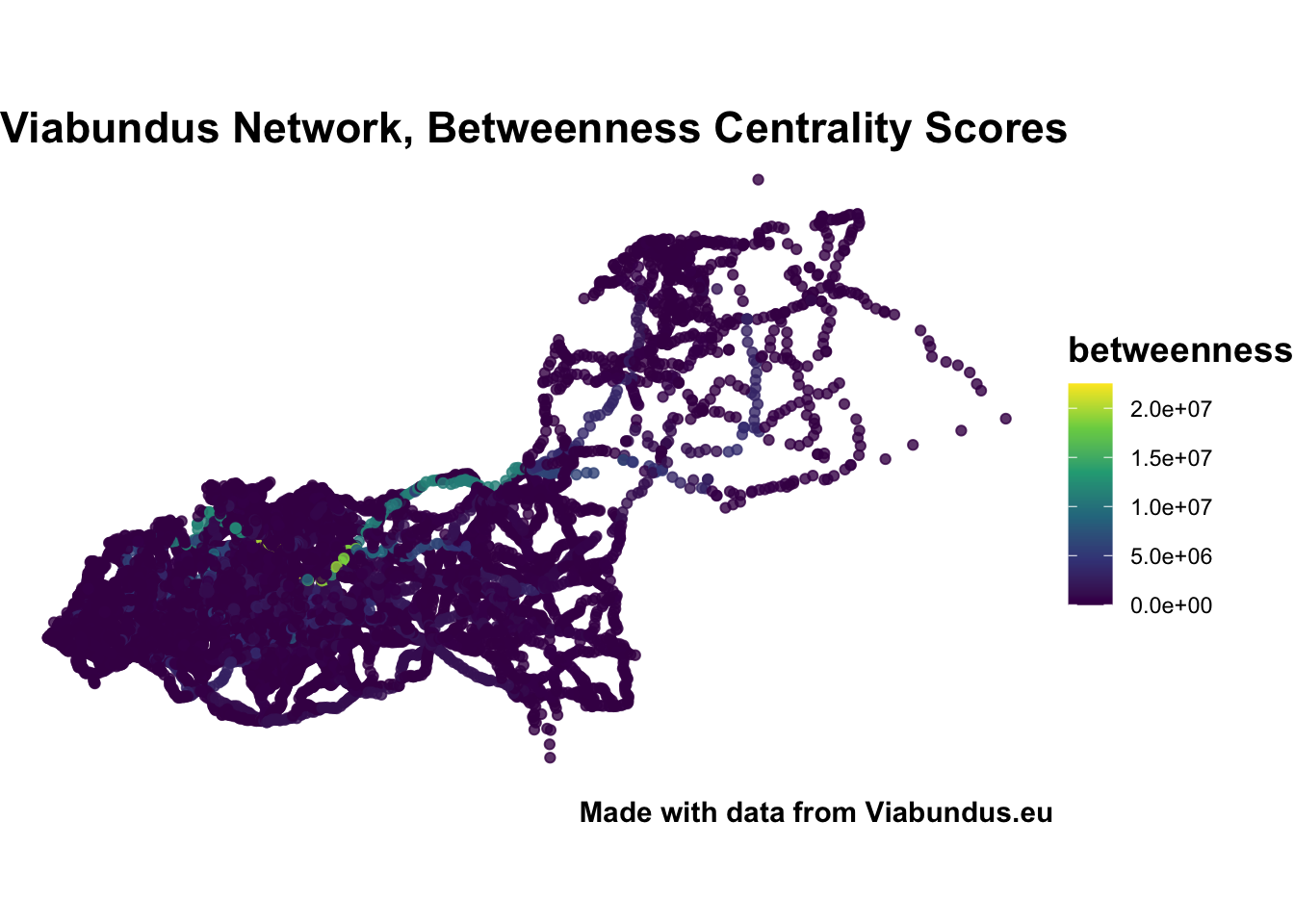
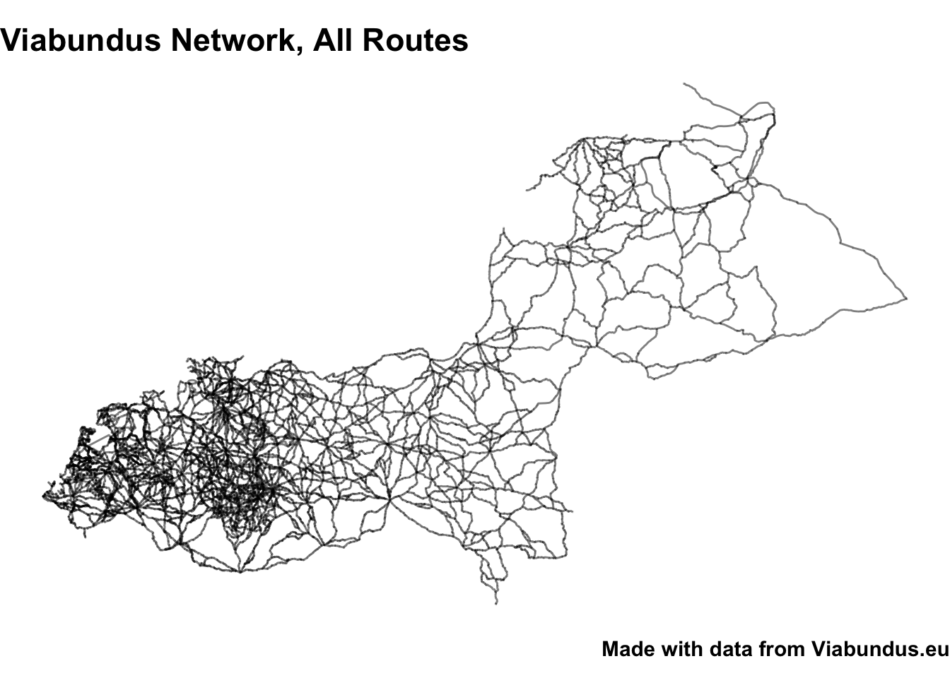
Interestingly, the highest betweenness nodes all seem to fall along a single path. Is this a particularly important trunk road? We can also plot the whole network. To use ggplot, create separate nodes and edges tables using as_tibble, and add them as separate geoms to the same plot:
ggplot() +
  geom_sf(data = sf_net %>% activate(nodes) %>% as_tibble(), alpha =  .1, size  = .01)  +
  geom_sf(data = sf_net %>% activate(edges) %>% as_tibble(), alpha = .5) +theme_void() +
  labs(title  = "Viabundus Network, All Routes", caption = 'Made with data from Viabundus.eu') +
  theme(title = element_text(size = 14, face = 'bold'))
Shortest-path calculation
The nicest application of these two resources I’ve found so far is to use sfnetworks to calculate the shortest path between any set of points in the network. This uses Dijkstra’s algorithm, along with the lengths of the spatial lines as weights (or impedance), to calculate the shortest route between any two points (or from one start point to a range of end points). This is done with the function st_shortest_paths.
st_network_paths takes from and to arguments, using the node ID from the nodes table. You’ll need to figure out some way to find the relevant node IDs to enter here—the most convenient way I’ve found is first to make a copy of just the nodes table:
nodes_lookup_table = sf_net %>% activate(nodes) %>% as_tibble()
The ID you need is the row index - create a column called node_id containing this info:
nodes_lookup_table = nodes_lookup_table %>% mutate(node_id = 1:nrow(.))
Looking at the table, you’ll see that sometimes the same place has been assigned to multiple closest coordinates. For now, I’m just going to pick the first one.
utrecht_node_id = nodes_lookup_table %>% filter(Name == 'Utrecht') %>% head(1) %>% pull(node_id)
hamburg_node_id = nodes_lookup_table %>% filter(Name == 'Hamburg') %>% head(1) %>% pull(node_id)
Run st_network_paths supplying the points you want to calculate the route between as from and to arguments:
paths = st_network_paths(sf_net, from =utrecht_node_id, to = hamburg_node_id)

paths
## # A tibble: 1 x 2
##   node_paths edge_paths
##   <list>     <list>
## 1 <int [99]> <int [98]>
The result of st_network_paths is a dataframe with two columns, each containing a vector of edge or node IDs. First convert each into a dataframe with a single columns of IDs:
 node_list = paths %>%
  slice(1) %>%
  pull(node_paths) %>%
  unlist() %>% as_tibble()

edge_list = paths %>%
  slice(1) %>%
  pull(edge_paths) %>%
  unlist() %>% as_tibble()
Use inner join() to attach the edge and node IDs in the route to the edge and nodes tables from the sfnetwork object. You’ll need to recreate them as sf objects:
line_to_draw = edge_list %>% inner_join(sf_net %>%
  activate(edges) %>%
  as_tibble() %>%
  mutate(edge_id = 1:nrow(.)) , by = c('value' = 'edge_id'))

line_to_draw = line_to_draw %>% st_as_sf()
line_to_draw = line_to_draw %>% st_set_crs(4326)

nodes_to_draw = node_list %>% inner_join(sf_net %>%
  activate(nodes) %>%
  as_tibble() %>%
  mutate(node_id = 1:nrow(.)) , by = c('value' = 'node_id'))

nodes_to_draw = nodes_to_draw %>% st_as_sf()
nodes_to_draw = nodes_to_draw %>% st_set_crs(4326)
Plot this using Leaflet:
library(leaflet)

leaflet() %>%
  addTiles() %>%
  addCircles(data = nodes_to_draw, label = ~Name) %>%
  addPolylines(data  = line_to_draw)
Constructing an itinerary using the node information
The paths object gives both the roads (edges/lines) and towns or other points of interest passed (nodes). We can use the additional data from the list of nodes to get more information on the route along the way.
First, it’s worth taking a closer look at the nodes data.
nodes_lookup_table %>% glimpse()
## Rows: 12,567
## Columns: 45
## $ WKT                     <POINT [°]> POINT (22.47944 58.24702), POINT (22.80…
## $ ID                      <dbl> 287, 7743, 6695, 3479, 5911, 7263, 10815, 386…
## $ Parent_ID               <dbl> NA, NA, NA, NA, NA, NA, 3865, NA, NA, NA, NA,…
## $ Name                    <chr> "Kuressaare", "Tõlluste", "Sakla", "Kahtla", …
## $ Alternative_Name        <chr> "Arensburg; Arnsborch; Arnburg; Arensburgk", …
## $ Geonames_ID             <dbl> 590939, 588249, 588839, 591760, 589398, 59043…
## $ Ready                   <chr> NA, NA, NA, NA, NA, NA, NA, NA, NA, NA, NA, N…
## $ Is_Settlement           <chr> "y", "y", "y", NA, "y", "y", NA, "y", "y", "y…
## $ Settlement_From         <dbl> 1384, 1528, 1645, NA, 1250, 1345, NA, 1532, 1…
## $ Settlement_To           <dbl> NA, NA, NA, NA, NA, NA, NA, NA, NA, NA, NA, N…
## $ Settlement_Description  <chr> "In the second half of the 14th century the c…
## $ Is_Town                 <chr> "y", NA, NA, NA, NA, NA, NA, NA, NA, NA, NA, …
## $ Town_From               <dbl> 1563, NA, NA, NA, NA, NA, NA, NA, NA, NA, NA,…
## $ Town_To                 <lgl> NA, NA, NA, NA, NA, NA, NA, NA, NA, NA, NA, N…
## $ Town_Description        <chr> "The settlement near the castle was granted R…
## $ Is_Toll                 <chr> NA, NA, NA, NA, NA, NA, NA, NA, NA, NA, NA, N…
## $ Toll_From               <dbl> NA, NA, NA, NA, NA, NA, NA, NA, NA, NA, NA, N…
## $ Toll_To                 <dbl> NA, NA, NA, NA, NA, NA, NA, NA, NA, NA, NA, N…
## $ Toll_Description        <chr> NA, NA, NA, NA, NA, NA, NA, NA, NA, NA, NA, N…
## $ Is_Staple               <chr> NA, NA, NA, NA, NA, NA, NA, NA, NA, NA, NA, N…
## $ Staple_From             <dbl> NA, NA, NA, NA, NA, NA, NA, NA, NA, NA, NA, N…
## $ Staple_To               <dbl> NA, NA, NA, NA, NA, NA, NA, NA, NA, NA, NA, N…
## $ Staple_Duration_Of_Stay <dbl> NA, NA, NA, NA, NA, NA, NA, NA, NA, NA, NA, N…
## $ Staple_Description      <chr> NA, NA, NA, NA, NA, NA, NA, NA, NA, NA, NA, N…
## $ Is_Fair                 <chr> NA, NA, NA, NA, NA, NA, NA, NA, NA, NA, NA, N…
## $ Fair_From               <dbl> NA, NA, NA, NA, NA, NA, NA, NA, NA, NA, NA, N…
## $ Fair_To                 <lgl> NA, NA, NA, NA, NA, NA, NA, NA, NA, NA, NA, N…
## $ Fair_Description        <chr> NA, NA, NA, NA, NA, NA, NA, NA, NA, NA, NA, N…
## $ Is_Ferry                <chr> NA, NA, NA, NA, NA, "y", "y", NA, NA, NA, NA,…
## $ Ferry_From              <dbl> NA, NA, NA, NA, NA, NA, NA, NA, NA, NA, NA, N…
## $ Ferry_To                <lgl> NA, NA, NA, NA, NA, NA, NA, NA, NA, NA, NA, N…
## $ Ferry_Description       <chr> NA, NA, NA, NA, NA, NA, NA, NA, NA, NA, NA, N…
## $ Is_Bridge               <chr> NA, NA, NA, NA, NA, NA, NA, NA, NA, NA, NA, N…
## $ Bridge_From             <dbl> NA, NA, NA, NA, NA, NA, NA, NA, NA, NA, NA, N…
## $ Bridge_To               <lgl> NA, NA, NA, NA, NA, NA, NA, NA, NA, NA, NA, N…
## $ Bridge_Description      <chr> NA, NA, NA, NA, NA, NA, NA, NA, NA, NA, NA, N…
## $ Is_Harbour              <chr> NA, NA, NA, NA, NA, NA, NA, NA, NA, NA, NA, N…
## $ Harbour_From            <dbl> NA, NA, NA, NA, NA, NA, NA, NA, NA, NA, NA, N…
## $ Harbour_To              <lgl> NA, NA, NA, NA, NA, NA, NA, NA, NA, NA, NA, N…
## $ Harbour_Description     <chr> NA, NA, NA, NA, NA, NA, NA, NA, NA, NA, NA, N…
## $ Is_Lock                 <lgl> NA, NA, NA, NA, NA, NA, NA, NA, NA, NA, NA, N…
## $ Lock_From               <lgl> NA, NA, NA, NA, NA, NA, NA, NA, NA, NA, NA, N…
## $ Lock_To                 <lgl> NA, NA, NA, NA, NA, NA, NA, NA, NA, NA, NA, N…
## $ Lock_Description        <lgl> NA, NA, NA, NA, NA, NA, NA, NA, NA, NA, NA, N…
## $ node_id                 <int> 1, 2, 3, 4, 5, 6, 7, 8, 9, 10, 11, 12, 13, 14…
There are a large number of types of node, including town, settlement, bridge, harbour, ferry, and lock. Using the types will help to plan out a proper itinerary for the route.
There’s also dates from/to fields for each type, which means we can draw up an itinerary for a specific time period. From what I can tell, the official Viabundus map takes into account the infrastructure types in the node list (locks, bridges and ferries etc) and draws up a route which would have used the correct network at a specified date, but I haven’t figured out how to do that yet.
The Viabundus data format is quite ‘wide,’ which makes it difficult to easily filter. Each place can be multiple types, with multiple start and end points. To make it easier to work with, I used pivot_longer to make the data long, in a couple of steps.
First, I turned all the From/To columns into a pair: one column for the type of node, and a second for the value:
nodes_to_draw = nodes_to_draw %>% map_df(rev) # The route is in reverse order - switch this around

long_data = nodes_to_draw %>% mutate(order = 1:nrow(.)) %>%
  pivot_longer(names_to = 'data_type' , values_to = 'value_of', cols =matches("From$|To$", ignore.case = F))

long_data %>% select(Name, data_type, value_of) %>% head(10) %>% kbl()%>%
  kable_styling(bootstrap_options = c("striped", "hover", "condensed"))
| Name | data\_type | value\_of |
|---|---|---|
| Hamburg | Settlement\_From | 831 |
| Hamburg | Settlement\_To | NA |
| Hamburg | Town\_From | 1150 |
| Hamburg | Town\_To | NA |
| Hamburg | Toll\_From | 1188 |
| Hamburg | Toll\_To | NA |
| Hamburg | Staple\_From | 1458 |
| Hamburg | Staple\_To | 1748 |
| Hamburg | Fair\_From | 1000 |
| Hamburg | Fair\_To | NA |
Next I used ifelse to filter the value column in a different way depending on whether it was a to date or a from date:
long_data  = long_data %>%
  mutate(date_type = ifelse(str_detect(data_type, "From$"), 'from', 'to')) %>%
  filter(date_type == 'from' & value_of < 1600 | data_type == 'to' & value_of >1600| is.na(value_of))
Using, this, we can easily list each place visited:
library(htmltools)
long_data %>% distinct(order, .keep_all = T) %>% select(order, Name) %>% filter(!is.na(Name)) %>% distinct(Name) %>% kbl() %>%
  kable_styling(bootstrap_options = c("striped", "hover", "condensed"))%>%
  scroll_box(height = "400px")
| Name |
|---|
| Hamburg |
| Ottensen |
| Blankenese |
| Buxtehude |
| Kammerbusch |
| Ahrenswohlde |
| Wangersen |
| Steddorf |
| Boitzen |
| Heeslingen |
| Zeven |
| Oldendorf (Zeven) |
| Steinfeld |
| Otterstedt |
| Ottersberg |
| Bassen |
| Borstel (Achim) |
| Achim (Weser) |
| Uphusen (Bremen) |
| Mahndorf (Bremen) |
| Arbergen |
| Hemelingen |
| Hastedt |
| Bremen |
| Neustadt |
| Warturm |
| Kirchhuchting |
| Mittelshuchting |
| Varrel |
| Horstedt |
| Wildeshausen |
| Ahlhorn |
| Lethe |
| Bethen |
| Cloppenburg |
| Krapendorf |
| Lastrup |
| Löningen |
| Haselünne |
| Bawinkel |
| Lingen |
| Schepsdorf |
| Südlohne (Bentheim) |
| Nordhorn |
| Ootmarsum |
| Almelo |
| Wierden |
| Rijssen |
| Heeten |
| Deventer |
| Twello |
| Apeldoorn |
| Hoog-Soeren |
| Garderen |
| Voorthuizen |
| Terschuur |
| Hoevelaken |
| Amersfoort |
| De Bilt |
| Utrecht |
Another useful task is to make a nice summary of the places visited and their types. To do this easily, the data needs to be made ‘longer’ again. This time, we want a pair of columns where one is the node type, and the other is whether it is a ‘y’ or simply empty.
longer_data = long_data %>% pivot_longer(names_to = 'node_type', values_to = 'type', cols = matches('^Is_'))

longer_data %>% select(Name, node_type, type) %>% head(10)
## # A tibble: 10 x 3
##    Name    node_type     type
##    <chr>   <chr>         <chr>
##  1 Hamburg Is_Settlement y
##  2 Hamburg Is_Town       y
##  3 Hamburg Is_Toll       y
##  4 Hamburg Is_Staple     y
##  5 Hamburg Is_Fair       y
##  6 Hamburg Is_Ferry      <NA>
##  7 Hamburg Is_Bridge     <NA>
##  8 Hamburg Is_Harbour    y
##  9 Hamburg Is_Lock       <NA>
## 10 Hamburg Is_Settlement y
You’ll notice that Hamburg now has multiple repeated entries for each of the types, because we had already duplicated the data in the previous step, when making the dates long. This will need to be fixed for counts.
First, filter out any entries where the type is NA (this means that particular place was not that type):
longer_data = longer_data %>% filter(!is.na(type))
Now we can add all the node types associated with each place, using summarise. We need to use unique too, and then it’ll just print one instance of each type for each place:
longer_data %>%
  group_by(order) %>%
  summarise(Name = max(Name),types = paste0(unique(node_type), collapse = '; ')) %>% filter(!is.na(Name)) %>% kbl()%>%
  kable_styling(bootstrap_options = c("striped", "hover", "condensed"))%>%
  scroll_box(height = "400px")
| order | Name | types |
|---|---|---|
| 1 | Hamburg | Is\_Settlement; Is\_Town; Is\_Toll; Is\_Staple; Is\_Fair; Is\_Harbour |
| 3 | Ottensen | Is\_Settlement |
| 4 | Blankenese | Is\_Settlement; Is\_Ferry |
| 6 | Buxtehude | Is\_Settlement; Is\_Town; Is\_Toll; Is\_Fair |
| 7 | Buxtehude | Is\_Settlement; Is\_Town; Is\_Toll; Is\_Fair |
| 8 | Buxtehude | Is\_Settlement; Is\_Town; Is\_Toll; Is\_Fair |
| 9 | Kammerbusch | Is\_Settlement |
| 10 | Ahrenswohlde | Is\_Settlement |
| 11 | Wangersen | Is\_Settlement |
| 12 | Steddorf | Is\_Settlement |
| 13 | Boitzen | Is\_Settlement |
| 14 | Heeslingen | Is\_Settlement |
| 15 | Zeven | Is\_Settlement; Is\_Fair |
| 16 | Zeven | Is\_Settlement; Is\_Fair |
| 17 | Oldendorf (Zeven) | Is\_Settlement |
| 18 | Steinfeld | Is\_Settlement |
| 19 | Otterstedt | Is\_Settlement |
| 20 | Ottersberg | Is\_Settlement; Is\_Toll; Is\_Fair |
| 21 | Bassen | Is\_Settlement |
| 22 | Borstel (Achim) | Is\_Settlement |
| 23 | Achim (Weser) | Is\_Settlement |
| 24 | Uphusen (Bremen) | Is\_Settlement |
| 25 | Mahndorf (Bremen) | Is\_Settlement |
| 26 | Arbergen | Is\_Settlement |
| 27 | Hemelingen | Is\_Settlement |
| 28 | Hastedt | Is\_Settlement |
| 29 | Bremen | Is\_Settlement; Is\_Town; Is\_Toll; Is\_Staple; Is\_Fair |
| 30 | Bremen | Is\_Settlement; Is\_Town; Is\_Toll; Is\_Staple; Is\_Fair |
| 33 | Warturm | Is\_Settlement; Is\_Toll; Is\_Bridge |
| 34 | Kirchhuchting | Is\_Settlement |
| 35 | Mittelshuchting | Is\_Settlement |
| 36 | Varrel | Is\_Settlement; Is\_Toll |
| 37 | Horstedt | Is\_Settlement |
| 38 | Wildeshausen | Is\_Settlement; Is\_Town; Is\_Toll; Is\_Fair |
| 39 | Wildeshausen | Is\_Settlement; Is\_Town; Is\_Toll; Is\_Fair |
| 40 | Wildeshausen | Is\_Settlement; Is\_Town; Is\_Toll; Is\_Fair |
| 41 | Ahlhorn | Is\_Settlement |
| 42 | Ahlhorn | Is\_Settlement |
| 43 | Lethe | Is\_Settlement |
| 44 | Bethen | Is\_Settlement |
| 45 | Cloppenburg | Is\_Settlement; Is\_Town; Is\_Toll; Is\_Fair |
| 46 | Cloppenburg | Is\_Settlement; Is\_Town; Is\_Toll; Is\_Fair |
| 47 | Cloppenburg | Is\_Settlement; Is\_Town; Is\_Toll; Is\_Fair |
| 48 | Krapendorf | Is\_Settlement |
| 49 | Krapendorf | Is\_Settlement |
| 50 | Lastrup | Is\_Settlement |
| 51 | Löningen | Is\_Settlement |
| 52 | Haselünne | Is\_Settlement; Is\_Town; Is\_Toll; Is\_Fair |
| 55 | Bawinkel | Is\_Settlement |
| 56 | Lingen | Is\_Settlement; Is\_Town; Is\_Fair |
| 57 | Lingen | Is\_Settlement; Is\_Town; Is\_Fair |
| 60 | Schepsdorf | Is\_Settlement |
| 61 | Schepsdorf | Is\_Settlement |
| 62 | Südlohne (Bentheim) | Is\_Settlement |
| 63 | Nordhorn | Is\_Settlement; Is\_Town; Is\_Toll |
| 64 | Nordhorn | Is\_Settlement; Is\_Town; Is\_Toll |
| 69 | Ootmarsum | Is\_Settlement; Is\_Town |
| 70 | Ootmarsum | Is\_Settlement; Is\_Town |
| 71 | Ootmarsum | Is\_Settlement; Is\_Town |
| 72 | Almelo | Is\_Settlement; Is\_Town |
| 73 | Almelo | Is\_Settlement; Is\_Town |
| 74 | Wierden | Is\_Settlement |
| 75 | Rijssen | Is\_Settlement; Is\_Town |
| 76 | Rijssen | Is\_Settlement; Is\_Town |
| 77 | Rijssen | Is\_Settlement; Is\_Town |
| 78 | Heeten | Is\_Settlement |
| 79 | Heeten | Is\_Settlement |
| 80 | Deventer | Is\_Settlement; Is\_Town |
| 81 | Deventer | Is\_Settlement; Is\_Town |
| 83 | Twello | Is\_Settlement |
| 84 | Twello | Is\_Settlement |
| 85 | Apeldoorn | Is\_Settlement; Is\_Toll |
| 86 | Hoog-Soeren | Is\_Settlement |
| 87 | Garderen | Is\_Settlement |
| 88 | Voorthuizen | Is\_Settlement |
| 89 | Voorthuizen | Is\_Settlement |
| 90 | Terschuur | Is\_Settlement |
| 91 | Hoevelaken | Is\_Settlement |
| 92 | Hoevelaken | Is\_Settlement |
| 93 | Amersfoort | Is\_Settlement; Is\_Town |
| 94 | Amersfoort | Is\_Settlement; Is\_Town |
| 95 | Amersfoort | Is\_Settlement; Is\_Town |
| 97 | De Bilt | Is\_Settlement |
| 98 | De Bilt | Is\_Settlement |
| 99 | Utrecht | Is\_Settlement; Is\_Town; Is\_Harbour |
Tidy data also allows us to count the totals for each type of node passed. Again, we want to remove the duplicated data which is easy to do with distinct
longer_data %>% distinct(order, node_type) %>% group_by(node_type) %>% tally() %>% kbl()%>%
  kable_styling(bootstrap_options = c("striped", "hover", "condensed"))
| node\_type | n |
|---|---|
| Is\_Bridge | 4 |
| Is\_Fair | 18 |
| Is\_Ferry | 3 |
| Is\_Harbour | 10 |
| Is\_Settlement | 85 |
| Is\_Staple | 3 |
| Is\_Toll | 20 |
| Is\_Town | 31 |
Estimate Travel Times
We can use this info on the nodes passed plus the road lengths to estimate the total travel time.
First, get the total distance (note that everything is in metres for now):
distance = line_to_draw %>% tally(Length) %>% pull(n)
Viabundus suggests 5km per hour for wagons, up to a maximum of 35km per day.
time_taken_in_hours = distance / 5000

time_taken_in_days = time_taken_in_hours/7
Passing through certain nodes slow you down, according to the Viabundus documentation. Staples forced merchants to stop for three days, and ferries add an hour for loading/unloading. We can use the lists generated above to add the correct time penalties:
staples = longer_data %>%
  distinct(order, node_type) %>%
  filter(node_type == 'Is_Staple') %>%
  tally() %>% pull(n)

ferries = longer_data %>%
  distinct(order, node_type) %>%
  filter(node_type == 'Is_Ferry') %>%
  tally() %>% pull(n)

ferries = ferries /24

total_time_taken = time_taken_in_days + staples+ ferries

paste0("Total time taken (in days): ", total_time_taken)
## [1] "Total time taken (in days): 15.3426"
Calculating all daily travel rates
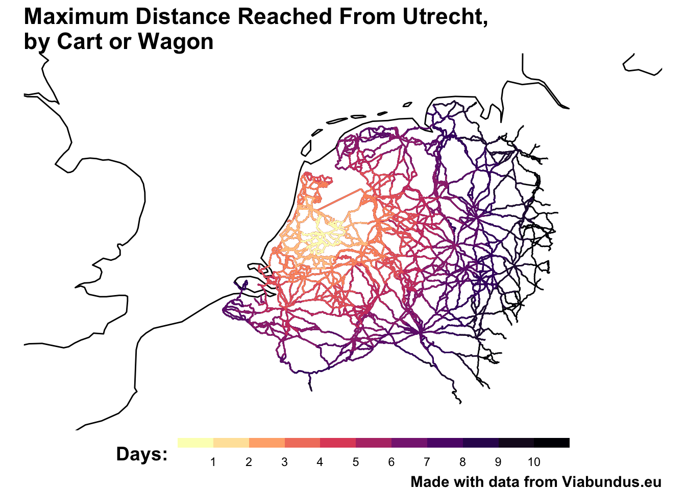
sfnetworks also has some functions for calculating the ‘neighbourhood’ of a node - the number of nodes reachable within a specified distance.
Using the code from the package vignette, I visualised the maximum one could travel from Utrecht in steps of a day for up to 10 days, ignoring staple stops:
Download a map of the world to use as a backdrop:
library(rnaturalearth)
library(rnaturalearthdata)

map = rnaturalearth::ne_coastline(returnclass = 'sf', scale = 'medium')
map = map %>% st_set_crs(4326)
Get a set of coordinates for Utrecht, in sf form:
utrecht_point = sf_net %>% activate(nodes) %>% filter(Name == 'Utrecht') %>%
  st_geometry() %>%
  st_combine() %>%
  st_centroid()
Make a list of the ‘thresholds’: a sequence of distances which will be fed to a for loop to calculate ten separate ‘neighborhood’ objects. The thresholds are each 35,000 metres long, corresponding to the maximum speed per day:
thresholds = rev(seq(0, 350000, 35000))
palette = sf.colors(n = 10)
Run the for loop, which will generate 10 separate network objects calculating the neighborhood of nodes from our starting point, and put them in a single list, with an additional ‘days’ column.
nbh = list()


for (i in c(1:10)) {
  nbh[[i]] = convert(sf_net, to_spatial_neighborhood, utrecht_point, thresholds[i])
   nbh[[i]] =  nbh[[i]] %>% st_set_crs(4326)
   nbh[[i]] = nbh[[i]] %>% activate(edges) %>% as_tibble() %>% mutate(days = 10-(i-1))

}
Use rbindlist() from data.table to merge them into one large spatial object:
library(data.table)
##
## Attaching package: 'data.table'

## The following objects are masked from 'package:dplyr':
##
##     between, first, last

## The following object is masked from 'package:purrr':
##
##     transpose
all_neighborhoods = rbindlist(nbh)
all_neighborhoods = st_as_sf(all_neighborhoods)
all_neighborhoods = all_neighborhoods %>% st_set_crs(4326)
Plot the results:
p = ggplot() +
  geom_sf(data = map) +
  geom_sf(data = all_neighborhoods, aes(color = days)) +
  coord_sf(xlim = c(0, 11), ylim = c(50, 54))+ theme_void() +
  labs(title  = "Maximum Distance Reached From Utrecht,\nby Cart or Wagon", color = 'Days:', caption = 'Made with data from Viabundus.eu') +
  theme(title = element_text(size = 14, face = 'bold')) +
  scale_color_viridis_c(direction = -1, option = 'A', breaks = 1:10) +
  guides(color = guide_colorsteps(barwidth = '20', barheight = .5)) +
  theme(legend.position = 'bottom')

p
Calculating elevation data
A few more R packages allow us to estimate the elevation travelled during the trip, which can also come in handy for understanding likely routes and travel times. Load the elevatr and slopes packages.
library(elevatr)
library(slopes)
Take the spatial lines data created above, and reverse it, because the path is reversed by default:
line_to_draw = line_to_draw %>% map_df(rev)

line_to_draw = line_to_draw %>% st_as_sf()
line_to_draw = line_to_draw %>% st_set_crs(4326)
The get_elev_raster function takes a different spatial object, called a SpatialLinesDataFrame. Create this using as('Spatial'):
sp_edges = line_to_draw %>% as('Spatial')
Now, download elevation data using get_elev_raster. This function takes the spatial object and downloads the relevant elevation data as a raster file from an online service. We can specify the zoom level (higher numbers mean a larger download) and the src, which is the data source, in this case Mapzen tiles hosted on Amazon Web Services.
elevation = get_elev_raster(sp_edges, z=9, src = "aws")
## Mosaicing & Projecting

## Note: Elevation units are in meters.
## Note: The coordinate reference system is:
##  GEOGCRS["WGS 84 (with axis order normalized for visualization)",
##     DATUM["World Geodetic System 1984",
##         ELLIPSOID["WGS 84",6378137,298.257223563,
##             LENGTHUNIT["metre",1]]],
##     PRIMEM["Greenwich",0,
##         ANGLEUNIT["degree",0.0174532925199433]],
##     CS[ellipsoidal,2],
##         AXIS["geodetic longitude (Lon)",east,
##             ORDER[1],
##             ANGLEUNIT["degree",0.0174532925199433,
##                 ID["EPSG",9122]]],
##         AXIS["geodetic latitude (Lat)",north,
##             ORDER[2],
##             ANGLEUNIT["degree",0.0174532925199433,
##                 ID["EPSG",9122]]]]
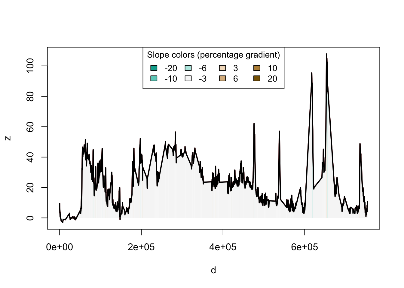
With this info, create a new ‘slope’ column using slope_raster and the raster we’ve just downloaded.
line_to_draw$slope = slope_raster(line_to_draw, e = elevation)
## Loading required namespace: geodist
Use the function slope_3d to estimate elevation data using the slopes, and add it as a Z axis to the lines sf object.
line_to_draw_3d = slope_3d(line_to_draw, elevation)
Plot the result using plot_slope:
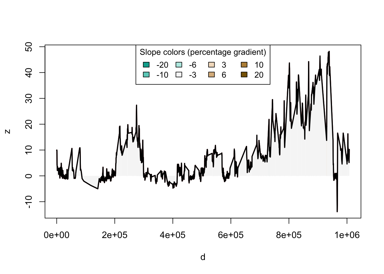
plot_slope(line_to_draw_3d, title = "Elevation Data, Utrecht to Hamburg")
Using Slope Data in the Shortest-Path Routing
We can also supply elevation data as part of the weight used by the shortest-path algorithm - letting us help an early modern trader avoid pesky hills. To do this, first download elevation data for the entire Viabundus dataset. I’ve reduced the zoom level a bit because it takes a long time to download and process.
all_elevation = get_elev_raster(edges_sf, z=7, src = "aws")
## Mosaicing & Projecting

## Note: Elevation units are in meters.
## Note: The coordinate reference system is:
##  GEOGCRS["WGS 84 (with axis order normalized for visualization)",
##     DATUM["World Geodetic System 1984",
##         ELLIPSOID["WGS 84",6378137,298.257223563,
##             LENGTHUNIT["metre",1]]],
##     PRIMEM["Greenwich",0,
##         ANGLEUNIT["degree",0.0174532925199433]],
##     CS[ellipsoidal,2],
##         AXIS["geodetic longitude (Lon)",east,
##             ORDER[1],
##             ANGLEUNIT["degree",0.0174532925199433,
##                 ID["EPSG",9122]]],
##         AXIS["geodetic latitude (Lat)",north,
##             ORDER[2],
##             ANGLEUNIT["degree",0.0174532925199433,
##                 ID["EPSG",9122]]]]
Use the full raster to get slope data for all the roads:
edges_sf$slope = slope_raster(edges_sf, e = all_elevation)
Create a new weight column in the roads dataset, taking the slope of each road into account using some kind of appropriate formula. I’ve done a very exaggerated one here, so we can easily see changes in the routing:
edges_sf = edges_sf %>% mutate(weight = Length + Length * (slope*1000))
Now, create an sfnetworks object and run the pathing algorithm as above:
sf_net_elev = as_sfnetwork(edges_sf, directed = F)

sf_net_elev = sf_net_elev %>%
  st_join(nodes_sf, join = st_nearest_feature)
## although coordinates are longitude/latitude, st_nearest_points assumes that they are planar
paths = st_network_paths(sf_net_elev, from =utrecht_node_id, to = hamburg_node_id)

 node_list = paths %>%
  slice(1) %>%
  pull(node_paths) %>%
  unlist() %>% as_tibble()

edge_list = paths %>%
  slice(1) %>%
  pull(edge_paths) %>%
  unlist() %>% as_tibble()

line_to_draw = edge_list %>% inner_join(sf_net %>%
  activate(edges) %>%
  as_tibble() %>%
  mutate(edge_id = 1:nrow(.)) , by = c('value' = 'edge_id'))

line_to_draw = line_to_draw %>% st_as_sf()
line_to_draw = line_to_draw %>% st_set_crs(4326)

nodes_to_draw = node_list %>% inner_join(sf_net %>%
  activate(nodes) %>%
  as_tibble() %>%
  mutate(node_id = 1:nrow(.)) , by = c('value' = 'node_id'))

nodes_to_draw = nodes_to_draw %>% st_as_sf()
nodes_to_draw = nodes_to_draw %>% st_set_crs(4326)
And plot it - it now takes a totally different route, avoiding the hills around Amerongen in the Netherlands, for example.
library(leaflet)

leaflet() %>%
  addTiles() %>%
  addCircles(data = nodes_to_draw, label = ~Name) %>%
  addPolylines(data  = line_to_draw)
Plot this in 3d to see the difference in elevation:
line_to_draw$slope = slope_raster(line_to_draw, e = all_elevation)


line_to_draw_3d = slope_3d(line_to_draw, all_elevation)

plot_slope(line_to_draw_3d, title = "Elevation Data, Utrecht to Hamburg")
Perhaps more useful would be to incorporate the slope data in figuring out the total journey lengths, by devising a formula and using it in the calculations above, but this is still an interesting application!
Conclusions
Viabundus is an amazing resource, and sfnetworks makes it super easy to import and work with the data. The project team should be immensely proud of the result, and I’m very grateful to them for releasing it as open access data.
Converting the files into a ‘tidy’ data structure where necessary helped me to more easily sort and filter results, which might be worth keeping in mind.
I can imagine this having lots of really interesting applications to understanding postal routes, itineraries, and so forth. Another way to use the data would be to link to geo-temporal events on Wikidata (such as battles and sieges), and estimate the routes travelled by individuals in EMLO by their letter dates and locations. This could be a good way of figuring out intermediate stops travelled, and through that the likelihood of them being caught up in certain events.
I’m also hoping to figure out how to correctly exclude certain nodes (or node types) when running the pathing algorithm (rather than just removing those nodes from the itinerary afterwards), perhaps by setting the weight of certain edges to Inf. This would make it possible to estimate a route which avoided tolls and staples, for example.
Hopefully, some day, we’ll have similar data for most of Europe. I look forward to further updates from the project!
Yann Ryan
Research Fellow, Networking Archives Project
I’ve been at Queen Mary, University of London since 2014 and recently completed a PhD in the history of early modern news.