Another feature to improve your data visualisations is to use interactive maps. Again, there are several ways to do this, including the package Leaflet.
The easiest way to create a map is with a package called tmap. This takes an sf object (similar to those we created in earlier weeks), and allows you to make a nice map using a syntax fairly similar to ggplot. Optionally, you can make these maps interactive.
To demonstrate this, I’ll use a dataset from the Shakespeare & Co project at Princeton, which contains information on the locations of members of the famous Shakespeare & Co bookshop and lending library in Paris.
First, install and load the tmap package.
library(tmap)
Warning: package 'tmap' was built under R version 4.5.1
library(tidyverse)
── Attaching core tidyverse packages ──────────────────────── tidyverse 2.0.0 ──
✔ dplyr 1.1.4 ✔ readr 2.1.5
✔ forcats 1.0.0 ✔ stringr 1.5.1
✔ ggplot2 3.5.2 ✔ tibble 3.3.0
✔ lubridate 1.9.4 ✔ tidyr 1.3.1
✔ purrr 1.0.4
── Conflicts ────────────────────────────────────────── tidyverse_conflicts() ──
✖ dplyr::filter() masks stats::filter()
✖ dplyr::lag() masks stats::lag()
ℹ Use the conflicted package (<http://conflicted.r-lib.org/>) to force all conflicts to become errors
Warning: Expected 2 pieces. Missing pieces filled with `NA` in 3 rows [1080, 1572,
2307].
Now, create an sf object, as we learned in previous weeks. This code converts the longitude and latitude columns to numeric, then filters out any NA values.
[basemaps] Tiles from "OpenStreetMap.Mapnik" at zoom level 3 couldn't be loaded
This message is displayed once per session.
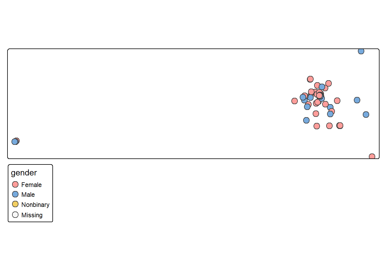
Use some options within tm_symbols to make the map more useful. Unlike ggplot, do not put them within aes(), and use quotation marks around the column names. size will determine the size of the points, either a column or a value. fill will determine the fill colour, again, either a column name or a colour name. id should point to a column in your data, which will appear as a label when a user hovers over your map. popup.vars should be given a vector of column names, which will then show when a point is clicked.
You can specify the zoom and starting point by adding the layer tm_options() and using the option set_view within it. This should list a vector of length 3 with the longitude, latitude, and zoom level:
tm_basemap('OpenStreetMap.Mapnik') +tm_shape(sco_data_sf) +tm_symbols(size = .75, id ="name", fill ='gender',popup.vars =c('name', 'gender', 'birth_year', 'death_year') ) +tm_options( set_view =c(2.34, 48.86, 11))
Interactive choropleth maps
To make nice interactive maps we’ll use another package called tmap. tmap is a very nice package specifically for making maps. Unfortunately it doesn’t use exactly the same syntax we have learned with ggplot, but it is by far the easiest way to make interactive maps.
The following code only works in RStudio so it is static in the book:
Load the tmap library.
Download a map from R Natural Earth
Switch to the ‘view’ mode using tmap_mode("view") to make the output an interactive map.
tm_shape() is more or less the equivalent of ggplot(): it’s the ‘base’ of the map, where we specify which shapefile should be used. On top of this we add layers, such as polygons or points, and also additional map elements such as a legend, scale, projection, and so forth. We can also add additional tm_shape() layers.
Add the tm_polygons() layer which will draw polygon shapes on the map based on the shapefile. Set the col to the income_grp column. Note the difference from ggplot - where we would set the fill, and the column name would not be in quotation marks. Set the id which will determine which column is used to display text with a mouse hover.
Add a tm_view() layer, which allows us to set options for the interactive viewer. Add a vector of three numbers: the starting latitude and longitude, and the zoom level.